Chapter 7 Wage Analytics
7.1 Introduction
The wage Analytics Division (WAD) has hired me as their new data scientist. My mission is to determine whether demographic and employment characteristics can be used to predict whether a worker earn a high or low wage. I will create a binary wage category, explore statistical relationships between variables, and build a logistic regression model capable of predicting wage level using demographic, job, and health-related information. I will help the company understand which characteristics are associated with higher earnings and evaluate how well a predictive model performs on unseen data.
For this assignment, the packages we will be using include: ISLR2, mosaic, tibble, dplyr, stringr, stats, rcompanion, caTools, pROC, and caret.
Here is the full report.
7.3 Step 2: Data Cleaning
7.3.1 Removing the numeric prefixes so only the category name remains in each column
WAD_Data<- WAD_Data %>%
  mutate(maritl=str_remove_all(maritl, "\\d+\\.?\\d*"))

WAD_Data<- WAD_Data %>%
  mutate(race=str_remove_all(race, "\\d+\\.?\\d*"))

WAD_Data<- WAD_Data %>%
  mutate(maritl=str_remove_all(maritl, "\\d+\\.?\\d*"))

WAD_Data<- WAD_Data %>%
  mutate(education=str_remove_all(education, "\\d+\\.?\\d*"))

WAD_Data<- WAD_Data %>%
  mutate(region=str_remove_all(region, "\\d+\\.?\\d*"))

WAD_Data<- WAD_Data %>%
  mutate(jobclass=str_remove_all(jobclass, "\\d+\\.?\\d*"))

WAD_Data<- WAD_Data %>%
  mutate(health=str_remove_all(health, "\\d+\\.?\\d*"))

WAD_Data<- WAD_Data %>%
  mutate(health_ins=str_remove_all(health_ins, "\\d+\\.?\\d*"))
7.4 Step 3: Classical Statistical Tests
7.4.1 T-test
I will be running a t-test comparing age between High and Low wage earners
##
##  Welch Two Sample t-test
##
## data:  age by WageCategory
## t = 11.143, df = 2724.7, p-value < 2.2e-16
## alternative hypothesis: true difference in means between group High and group Low is not equal to 0
## 95 percent confidence interval:
##  3.851525 5.496555
## sample estimates:
## mean in group High  mean in group Low
##           44.68510           40.01106
Mean age of high wage earners: 44.69
Mean age of low wage earners: 40.01
T-statistic: 11.14
df: 2724.2
p-value: 2.2e-16
A t-test was conducted to compare age between high and low wage earners. Results shown a significant difference in age between high and low wage earners, meaning age differs between wage categories.
7.4.2 ANOVA Test
I will be running an ANOVA comparing wages and education
##               Df  Sum Sq Mean Sq F value Pr(>F)
## education      4 1226364  306591   229.8 <2e-16 ***
## Residuals   2995 3995721    1334
## ---
## Signif. codes:  0 '***' 0.001 '**' 0.01 '*' 0.05 '.' 0.1 ' ' 1
F-statistic: 229.8
df1 & df2: 4, 2995
P-Value: 0 (significant)
An ANOVA was conducted to compare wages to education categories. Results showed a significant result of wages on education, meaning wages do differ across education categories.
7.5 Chi-Square Test
I will be running a chi-square test to compare wages and job class
##
##         Industrial  Information
##   High         629          854
## Low 878 569##
## Pearson's Chi-squared test with Yates' continuity correction
##
## data: freq_table
## X-squared = 97.065, df = 1, p-value < 2.2e-16## Cramer V
## 0.1827χ²: 97.07
df: 1
P-value: <2.2e-16
Cramer’s V: 0.18
In our contingency table, high wage workers look like they are more likely to be in the information job class than the industry job class, while low wage workers look likely are more likely to be in the industry job class than the information job class.
7.6 Step 4: Logistic Regression Model
7.6.2 Logistic Regression Model
train_model <- glm(WageCategory ~ age + race + education + jobclass,
                   family = "binomial", data = training_data)

summary(train_model)
##
## Call:
## glm(formula = WageCategory ~ age + race + education + jobclass,
## family = "binomial", data = training_data)
##
## Coefficients:
## Estimate Std. Error z value Pr(>|z|)
## (Intercept) 2.935185 0.343237 8.551 < 2e-16 ***
## age -0.037335 0.004535 -8.233 < 2e-16 ***
## race Black 0.764835 0.274289 2.788 0.0053 **
## race Other 0.777147 0.589342 1.319 0.1873
## race White 0.100065 0.220999 0.453 0.6507
## education Advanced Degree -3.057636 0.255823 -11.952 < 2e-16 ***
## education College Grad -2.225714 0.217231 -10.246 < 2e-16 ***
## education HS Grad -0.667095 0.204373 -3.264 0.0011 **
## education Some College -1.508319 0.211860 -7.119 1.08e-12 ***
## jobclass Information -0.217930 0.104461 -2.086 0.0370 *
## ---
## Signif. codes: 0 '***' 0.001 '**' 0.01 '*' 0.05 '.' 0.1 ' ' 1
##
## (Dispersion parameter for binomial family taken to be 1)
##
## Null deviance: 2843.0 on 2050 degrees of freedom
## Residual deviance: 2340.9 on 2041 degrees of freedom
## AIC: 2360.9
##
## Number of Fisher Scoring iterations: 4Age was a significant predictor of the wage category along with education, and race. Job class seemed to not be a significant predictor of the wage category. Together, demographic characteristics show significant predictors of the wage category.
7.6.3 Odds ratios
##               (Intercept)                       age                race Black                race Other
##               18.82498568                0.96335380                2.14863936                2.17525697
##                race White education Advanced Degree    education College Grad         education HS Grad
##                1.10524309                0.04699865                0.10799030                0.51319738
##    education Some College      jobclass Information
##                0.22128161                0.80418153
7.7 Step 5: Model Evaluation on Test Data
7.7.3 Confusion Matrix
conf_matrix <-confusionMatrix(test_data$pred_class, test_data$WageCategory, positive = "High")
conf_matrix
## Confusion Matrix and Statistics
##
## Reference
## Prediction High Low
## High 124 301
## Low 321 133
##
## Accuracy : 0.2924
## 95% CI : (0.2625, 0.3237)
## No Information Rate : 0.5063
## P-Value [Acc > NIR] : 1.0000
##
## Kappa : -0.4147
##
## Mcnemar's Test P-Value : 0.4462
##
## Sensitivity : 0.2787
## Specificity : 0.3065
## Pos Pred Value : 0.2918
## Neg Pred Value : 0.2930
## Prevalence : 0.5063
## Detection Rate : 0.1411
## Detection Prevalence : 0.4835
## Balanced Accuracy : 0.2926
##
## 'Positive' Class : High
## 7.7.4 ROC Curve + AUC value
## Setting direction: controls < cases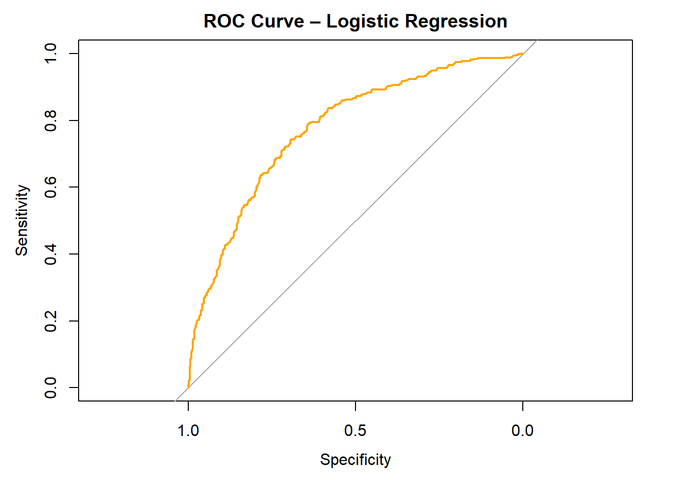
## Area under the curve: 0.7756Accuracy: 0.29 (accuracy is 29%)
Sensitivity: 0.27 (sensitivity is 27%)
Specificity: 0.31 (specificity is 31%)
Balanced Accuracy: 0.29 (balance accuracy is 29%)
The ROC curve has an AUC of 0.77, indicating model has a good ability to discriminate although accuracy is pretty low (29%)
Compared to the no information rate, the model performs worse than random guessing.
The model doesnt identify high earners well due to the sensitivity being low (27%) which means is misses high wage earners.
7.8 Step 6: Final Interpretation
When we performed the t-test comparing wage to age, a significant result was shown, meaning that age was meaningfully related to wage. When an ANOVA test was conducted comparing wages and education, a significant result was shown, meaning that education was meaningfully related to wage. When a chi-square was performed comparing wages and jobclass, a significant result was shown, meaning that age was meaningfully related to wage.
The following variables were significant predictors in the logistic regression model: Age, Education, and Race. The model did not perform well with unseen data because accuracy was only 29% compared to 51% rate with no prior information, meaning that the model was not as accurate as we expected. The wage group the model predicted best was high wages. If I were to repeat this analysis, I would add marital status and remove age.