Chapter 5 Florida Crime Assignment
5.1 Introduction
The Florida Police Department has hired me as their new data analyst. The mission is to uncover what socioeconomic factors are most strongly associated with rising crime rates across Florida counties. The Florida Police Department is particularly interested in whether income, education, or urbanization play the largest role in explaining differences in crime rates.
For this assignment, the packages we will be using include: readxl, tidyverse, dplyr, stringr, skimr, ggplot2, patchwork, Hmisc, ggcorrplot, and broom.
5.2 Step 1: Loading and Preparing the data
5.2.2 Cleaning the data
We will be renaming the columns to: Crime, Income, HighSchoolGrad, and UrbanPop and making sure all county names are formatted so that only the first letter is capitalized.
Florida_Data<- Florida_Data %>%
  rename(
    Crime= C,
    Income= I,
    HighSchoolGrad= HS,
    UrbanPop=U
  )

Florida_Data<-Florida_Data %>%
  mutate(County=str_to_title(County))

Florida_Data
## # A tibble: 67 × 5
## County Crime Income HighSchoolGrad UrbanPop
## <chr> <dbl> <dbl> <dbl> <dbl>
## 1 Alachua 104 22.1 82.7 73.2
## 2 Baker 20 25.8 64.1 21.5
## 3 Bay 64 24.7 74.7 85
## 4 Bradford 50 24.6 65 23.2
## 5 Brevard 64 30.5 82.3 91.9
## 6 Broward 94 30.6 76.8 98.9
## 7 Calhoun 8 18.6 55.9 0
## 8 Charlotte 35 25.7 75.7 80.2
## 9 Citrus 27 21.3 68.6 31
## 10 Clay 41 34.9 81.2 65.8
## # ℹ 57 more rows5.2.3 Inspect and summarize data set
Next we will inspect and summarize the dataset
## tibble [67 × 5] (S3: tbl_df/tbl/data.frame)
##  $ County        : chr [1:67] "Alachua" "Baker" "Bay" "Bradford" ...
##  $ Crime         : num [1:67] 104 20 64 50 64 94 8 35 27 41 ...
##  $ Income        : num [1:67] 22.1 25.8 24.7 24.6 30.5 30.6 18.6 25.7 21.3 34.9 ...
##  $ HighSchoolGrad: num [1:67] 82.7 64.1 74.7 65 82.3 76.8 55.9 75.7 68.6 81.2 ...
## $ UrbanPop : num [1:67] 73.2 21.5 85 23.2 91.9 98.9 0 80.2 31 65.8 ...| Name | Florida_Data |
| Number of rows | 67 |
| Number of columns | 5 |
| _______________________ | |
| Column type frequency: | |
| character | 1 |
| numeric | 4 |
| ________________________ | |
| Group variables | None |
Variable type: character
| skim_variable | n_missing | complete_rate | min | max | empty | n_unique | whitespace |
|---|---|---|---|---|---|---|---|
| County | 0 | 1 | 3 | 9 | 0 | 67 | 0 |
Variable type: numeric
| skim_variable | n_missing | complete_rate | mean | sd | p0 | p25 | p50 | p75 | p100 | hist |
|---|---|---|---|---|---|---|---|---|---|---|
| Crime | 0 | 1 | 52.40 | 28.19 | 0.0 | 35.50 | 52.0 | 69.00 | 128.0 | ▃▇▇▃▂ |
| Income | 0 | 1 | 24.51 | 4.68 | 15.4 | 21.05 | 24.6 | 28.15 | 35.6 | ▂▇▅▅▂ |
| HighSchoolGrad | 0 | 1 | 69.49 | 8.86 | 54.5 | 62.45 | 69.0 | 76.90 | 84.9 | ▇▇▆▇▆ |
| UrbanPop | 0 | 1 | 49.56 | 33.97 | 0.0 | 21.60 | 44.6 | 83.55 | 99.6 | ▅▆▂▃▇ |
5.3 Step 2: Exploratory Data Analysis
We will now compute basic descriptive statistics.
##     County              Crime           Income      HighSchoolGrad     UrbanPop
##  Length:67          Min.   :  0.0   Min.   :15.40   Min.   :54.50   Min.   : 0.00
##  Class :character   1st Qu.: 35.5   1st Qu.:21.05   1st Qu.:62.45   1st Qu.:21.60
##  Mode  :character   Median : 52.0   Median :24.60   Median :69.00   Median :44.60
##                     Mean   : 52.4   Mean   :24.51   Mean   :69.49   Mean   :49.56
##                     3rd Qu.: 69.0   3rd Qu.:28.15   3rd Qu.:76.90   3rd Qu.:83.55
##                     Max.   :128.0   Max.   :35.60   Max.   :84.90   Max.   :99.60
Using this simple code, we get the minimum, median, mean, and maximum of each column.
For Crime: Mean= 52.4, Median= 52, Range= 0-128
For Income: Mean= 24.51, Median= 24.60, Range= 15.40-35.60
For HighSchoolGrad: Mean= 54.50, Median= 69, Range= 54.50-84.90
For UrbanPop: Mean= 49.56, Median= 44.60, Range= 0-99.60
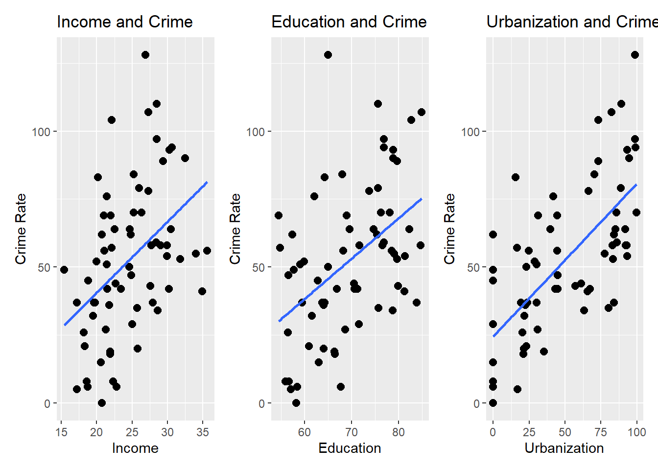
Next we will create three scatterplots below
5.3.1 Visual 1: Income and Crime
Visual_1<- ggplot(Florida_Data, aes(x=Income, y=Crime))+
  geom_point(size=2.5)+
  geom_smooth(method = "lm", se=FALSE) +
  labs(
    title = "Income and Crime",
    x="Income",
    y="Crime Rate"
  )
Visual_1
## `geom_smooth()` using formula = 'y ~ x'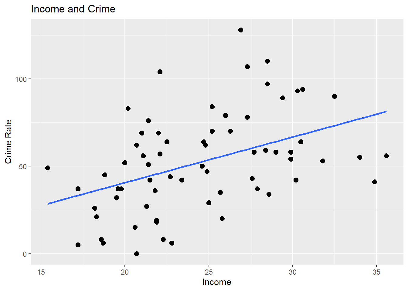
Figure 5.1: Plot graph showing income by crime since visualizing helps us see the trend
As income increases, crime rate increases.
5.3.2 Visual 2: Education and crime
Visual_2<- ggplot(Florida_Data, aes(x=HighSchoolGrad, y=Crime))+
  geom_point(size=2.5)+
  geom_smooth(method = "lm", se=FALSE) +
  labs(
    title = "Education and Crime",
    x="Education",
    y="Crime Rate"
  )
Visual_2
## `geom_smooth()` using formula = 'y ~ x'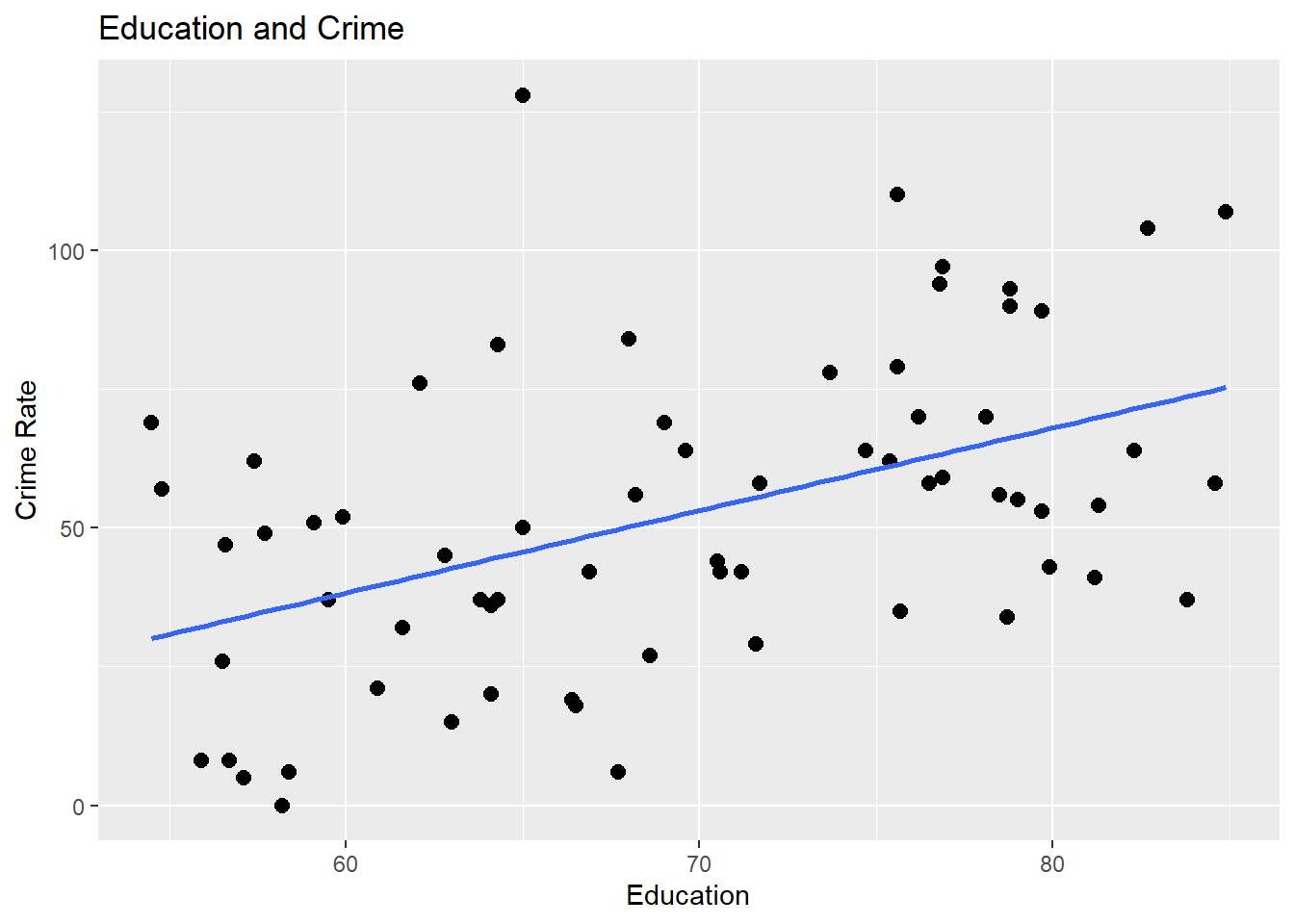
Figure 5.2: Plot graph showing education by crime since visualizing helps us see the trend
As education increases, crime rate increases.
5.3.3 Visual 3: Urbanization and Crime
Visual_3<- ggplot(Florida_Data, aes(x=UrbanPop, y=Crime))+
  geom_point(size=2.5)+
  geom_smooth(method = "lm", se=FALSE) +
  labs(
    title = "Urbanization and Crime",
    x="Urbanization",
    y="Crime Rate"
  )
Visual_3
## `geom_smooth()` using formula = 'y ~ x'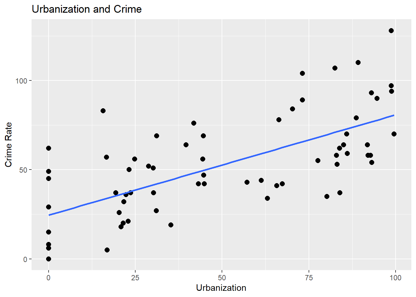
Figure 5.3: Graph plot showing urbainization by crime since visualizing helps us see the trend
As urbanization increases, crime rate increases.
5.4 Step 3: Correlation Analysis
We will be investigating which factors are most strongly correlated with crime.
5.4.1 Computing Correlation Matrix
Numeric_Florida_Data<- Florida_Data %>%
  select(Crime, Income, HighSchoolGrad, UrbanPop)
view(Numeric_Florida_Data)

Correlation_Matrix<-rcorr(as.matrix(Numeric_Florida_Data))
Correlation_Matrix
## Crime Income HighSchoolGrad UrbanPop
## Crime 1.00 0.43 0.47 0.68
## Income 0.43 1.00 0.79 0.73
## HighSchoolGrad 0.47 0.79 1.00 0.79
## UrbanPop 0.68 0.73 0.79 1.00
##
## n= 67
##
##
## P
## Crime Income HighSchoolGrad UrbanPop
## Crime 2e-04 0e+00 0e+00
## Income 2e-04 0e+00 0e+00
## HighSchoolGrad 0e+00 0e+00 0e+00
## UrbanPop 0e+00 0e+00 0e+00Interpreting each relationship:
Income x Crime: 0.43. As income increases, crime increases (Positive-Weak)
Education x Crime: 0.47. As Education increases, crime increases. (Positive-Weak)
Urbanization x Crime: 0.68. As urbanization increases, crime increases. (Positive-Strongish)
The variable that shows the strongest relationship with Crime is UrbanPop(Urbanization).
5.5 Step 4: Building Regression Models
5.5.1 Building simple regression models
##
## Call:
## lm(formula = Crime ~ Income, data = Numeric_Florida_Data)
##
## Residuals:
##     Min      1Q  Median      3Q     Max
## -42.452 -21.347  -3.102  17.580  69.357
##
## Coefficients:
##             Estimate Std. Error t value Pr(>|t|)
## (Intercept) -11.6059    16.7863  -0.691 0.491782
## Income        2.6115     0.6729   3.881 0.000246 ***
## ---
## Signif. codes:  0 '***' 0.001 '**' 0.01 '*' 0.05 '.' 0.1 ' ' 1
##
## Residual standard error: 25.6 on 65 degrees of freedom
## Multiple R-squared:  0.1881, Adjusted R-squared:  0.1756
## F-statistic: 15.06 on 1 and 65 DF, p-value: 0.0002456## [1] 628.6045##
## Call:
## lm(formula = Crime ~ HighSchoolGrad, data = Numeric_Florida_Data)
##
## Residuals:
## Min 1Q Median 3Q Max
## -43.74 -21.36 -4.82 17.42 82.27
##
## Coefficients:
## Estimate Std. Error t value Pr(>|t|)
## (Intercept) -50.8569 24.4507 -2.080 0.0415 *
## HighSchoolGrad 1.4860 0.3491 4.257 6.81e-05 ***
## ---
## Signif. codes: 0 '***' 0.001 '**' 0.01 '*' 0.05 '.' 0.1 ' ' 1
##
## Residual standard error: 25.12 on 65 degrees of freedom
## Multiple R-squared: 0.218, Adjusted R-squared: 0.206
## F-statistic: 18.12 on 1 and 65 DF, p-value: 6.806e-05## [1] 626.0932##
## Call:
## lm(formula = Crime ~ UrbanPop, data = Numeric_Florida_Data)
##
## Residuals:
## Min 1Q Median 3Q Max
## -34.766 -16.541 -4.741 16.521 49.632
##
## Coefficients:
## Estimate Std. Error t value Pr(>|t|)
## (Intercept) 24.54125 4.53930 5.406 9.85e-07 ***
## UrbanPop 0.56220 0.07573 7.424 3.08e-10 ***
## ---
## Signif. codes: 0 '***' 0.001 '**' 0.01 '*' 0.05 '.' 0.1 ' ' 1
##
## Residual standard error: 20.9 on 65 degrees of freedom
## Multiple R-squared: 0.4588, Adjusted R-squared: 0.4505
## F-statistic: 55.11 on 1 and 65 DF, p-value: 3.084e-10## [1] 601.435.5.2 Building Multiple Regression Models
##
## Call:
## lm(formula = Crime ~ Income + HighSchoolGrad, data = Numeric_Florida_Data)
##
## Residuals:
##    Min     1Q Median     3Q    Max
## -42.75 -19.61  -4.57  18.52  77.86
##
## Coefficients:
##                Estimate Std. Error t value Pr(>|t|)
## (Intercept)    -46.1094    24.9723  -1.846   0.0695 .
## Income           1.0311     1.0839   0.951   0.3450
## HighSchoolGrad   1.0540     0.5729   1.840   0.0705 .
## ---
## Signif. codes:  0 '***' 0.001 '**' 0.01 '*' 0.05 '.' 0.1 ' ' 1
##
## Residual standard error: 25.14 on 64 degrees of freedom
## Multiple R-squared:  0.2289, Adjusted R-squared:  0.2048
## F-statistic: 9.5 on 2 and 64 DF, p-value: 0.000244## [1] 627.1524##
## Call:
## lm(formula = Crime ~ Income + UrbanPop, data = Numeric_Florida_Data)
##
## Residuals:
## Min 1Q Median 3Q Max
## -36.130 -15.590 -6.484 16.595 48.921
##
## Coefficients:
## Estimate Std. Error t value Pr(>|t|)
## (Intercept) 39.9723 16.3536 2.444 0.0173 *
## Income -0.7906 0.8049 -0.982 0.3297
## UrbanPop 0.6418 0.1110 5.784 2.36e-07 ***
## ---
## Signif. codes: 0 '***' 0.001 '**' 0.01 '*' 0.05 '.' 0.1 ' ' 1
##
## Residual standard error: 20.91 on 64 degrees of freedom
## Multiple R-squared: 0.4669, Adjusted R-squared: 0.4502
## F-statistic: 28.02 on 2 and 64 DF, p-value: 1.815e-09## [1] 602.4276##
## Call:
## lm(formula = Crime ~ Income + HighSchoolGrad + UrbanPop, data = Numeric_Florida_Data)
##
## Residuals:
## Min 1Q Median 3Q Max
## -35.407 -15.080 -6.588 16.178 50.125
##
## Coefficients:
## Estimate Std. Error t value Pr(>|t|)
## (Intercept) 59.7147 28.5895 2.089 0.0408 *
## Income -0.3831 0.9405 -0.407 0.6852
## HighSchoolGrad -0.4673 0.5544 -0.843 0.4025
## UrbanPop 0.6972 0.1291 5.399 1.08e-06 ***
## ---
## Signif. codes: 0 '***' 0.001 '**' 0.01 '*' 0.05 '.' 0.1 ' ' 1
##
## Residual standard error: 20.95 on 63 degrees of freedom
## Multiple R-squared: 0.4728, Adjusted R-squared: 0.4477
## F-statistic: 18.83 on 3 and 63 DF, p-value: 7.823e-09## [1] 603.67645.5.3 Comparing all models based on R squared, adjusted R squared, and AIC.
m1: Model 1 has a R square of 0.19, adjusted r square of 0.18, and an AIC of 628.60. 18% of the variance the model explains.
m2: Model 2 has a R square of 0.22, adjusted r square of 0.20, and an AIC of 626.09. 20% of the variance the model explains.
m3: Model 3 has a R square of 0.46, adjusted r square of 0.45, and an AIC of 601.43. 45% of the variance the model explains.
m4: Model 4 has a R square of 0.23, adjusted r square of 0.20, and an AIC of 627.15. 20% of the variance the model explains.
m5: Model 5 has a R square of 0.47, adjusted r square of 0.45, and an AIC of 602.43. 45% of the variance the model explains.
m6: Model 6 has a R square of 0.47, adjusted r square of 0.45, and an AIC of 603.68. 45% of the variance the model explains.
Model 3, 5, and 6 has an adjusted r square of 0.45 but different AIC. Model 3 AIC is 601.43, Model 5 AIC is 602.43, and Model 6 AIC is 603.68. Model 3 has the lowest AIC, therfore Model 3 (Crime and urbanization) is the model that best balances accuracy and simplicity.
5.6 Step 5: Findings
Dear Chief of the Florida Police Department,
The best model for predicting crime rates is model 3 (Crime~Urbanization), with the most influential predictor being Urbanization. 45% of the variance, the model explains. I recommend focusing on more urbanized areas to reduce crime rates because more urbanized areas experience higher rates of crime. One limitation of this analysis is that correlation does not equal causation. Just because there was a strongish correlation between crime and urbanization, does not mean that one causes the other. I would recommend into consideration my memo, but taking into consideration other factors that may contribute to high crime rates.