Chapter 3 Law Firm Analysis Part Two
3.1 Introduction
Hello! We are working as data scientists for a law firm analyzing NYC violation data. The NYC violation data can be found here The firm who hired us for this task wants to uncover hidden patterns in the data to inform their marketing strategy.
So far we have examined patterns by day of the week, time of day, and violation type. The firm wants us to do further investigation by exploring three questions:
Do certain agencies issue higher payments?
Do drivers from different states (NY, NJ, CT) pay more?
Do certain counties tend to have higher payment amounts?
The packages we will be using for this section include: tidyverse, httr, mosaic, supernova, jsonlite, AICmodavg, tidyr, dplyr, ggplot2, and supernova.
3.3 Data cleaning
In this step, we will now clean the county column to replace any abbreviations with the full county names
camera<-camera %>%
  mutate(county=case_when(
    county=="Q" ~"Queens County",
    county=="Qns" ~"Queens County",
    county=="QN" ~"Queens County",
    county=="K"~"Kings County",
    county=="BK"~"Kings County",
    county=="Kings"~"Kings County",
    county=="NY"~"New York County",
    county=="BX"~"Bronx County",
    county=="Bronx"~"Bronx County",
    county=="R"~"Richmond County",
    county=="RICH"~"Richmond County",
    county=="ST"~"Staten Island County",
     county=="MN"~"Monroe County",
    TRUE~county
))3.4 Question 1: Do certain agencies issue higher payments?
3.4.1 Descriptive Statistics
Agency_Statistics<- favstats(payment_amount ~ issuing_agency, data = camera) %>% arrange(desc(mean))

Agency_Statistics
## issuing_agency min Q1 median Q3 max mean sd n
## 1 HEALTH DEPARTMENT POLICE 243.81 243.810 243.81 243.8100 243.81 243.81000 NA 1
## 2 SEA GATE ASSOCIATION POLICE 190.00 190.000 190.00 190.0000 190.00 190.00000 0.00000 2
## 3 FIRE DEPARTMENT 180.00 180.000 180.00 180.0000 180.00 180.00000 NA 1
## 4 NYS OFFICE OF MENTAL HEALTH POLICE 0.00 180.000 180.00 190.0000 210.00 161.33333 65.99423 15
## 5 ROOSEVELT ISLAND SECURITY 0.00 135.000 180.00 190.0000 246.68 149.16083 90.57967 24
## 6 PORT AUTHORITY 0.00 180.000 180.00 190.0000 242.76 147.35792 82.58394 48
## 7 NYS PARKS POLICE 0.00 45.000 180.00 190.0000 242.58 143.86176 89.24158 34
## 8 PARKS DEPARTMENT 0.00 90.000 180.00 190.0000 245.28 128.47736 78.92728 144
## 9 TAXI AND LIMOUSINE COMMISSION 125.00 125.000 125.00 125.0000 125.00 125.00000 NA 1
## 10 HEALTH AND HOSPITAL CORP. POLICE 0.00 0.000 180.00 190.0000 245.64 124.71373 98.60130 51
## 11 POLICE DEPARTMENT 0.00 0.000 180.00 190.0000 260.00 123.93855 88.00388 214
## 12 CON RAIL 0.00 0.000 95.00 228.8875 243.87 112.62000 124.87146 6
## 13 DEPARTMENT OF TRANSPORTATION 0.00 50.000 75.00 125.0000 690.04 99.52822 82.88394 87273
## 14 TRAFFIC 0.00 65.000 115.00 115.0000 245.79 94.59362 44.47453 12091
## 15 OTHER/UNKNOWN AGENCIES 0.00 40.115 80.23 120.3450 160.46 80.23000 113.46235 2
## 16 TRANSIT AUTHORITY 0.00 0.000 75.00 125.0000 190.00 78.00000 82.05181 5
## 17 SUNY MARITIME COLLEGE 65.00 65.000 65.00 65.0000 65.00 65.00000 NA 1
## 18 NYC OFFICE OF THE SHERIFF 0.00 28.750 57.50 86.2500 115.00 57.50000 81.31728 2
## 19 DEPARTMENT OF SANITATION 0.00 0.000 65.00 105.0000 115.00 56.78571 48.26239 14
## 20 LONG ISLAND RAILROAD 0.00 0.000 0.00 0.0000 0.00 0.00000 NA 1
## missing
## 1 0
## 2 0
## 3 0
## 4 0
## 5 0
## 6 0
## 7 0
## 8 0
## 9 0
## 10 0
## 11 0
## 12 0
## 13 0
## 14 0
## 15 0
## 16 0
## 17 0
## 18 0
## 19 0
## 20 03.4.2 Inferential Statistics
##                   Df    Sum Sq Mean Sq F value Pr(>F)
## issuing_agency    19    937675   49351   7.858 <2e-16 ***
## Residuals      99910 627464684    6280
## ---
## Signif. codes:  0 '***' 0.001 '**' 0.01 '*' 0.05 '.' 0.1 ' ' 1
## 69 observations deleted due to missingness## Refitting to remove 69 cases with missing value(s)
## ℹ aov(formula = payment_amount ~ issuing_agency, data = listwise_delete(camera,
## c("payment_amount", "issuing_agency")))## Analysis of Variance Table (Type III SS)
## Model: payment_amount ~ issuing_agency
##
## SS df MS F PRE p
## ----- --------------- | ------------- ----- --------- ----- ----- -----
## Model (error reduced) | 937675.432 19 49351.339 7.858 .0015 .0000
## Error (from model) | 627464683.951 99910 6280.299
## ----- --------------- | ------------- ----- --------- ----- ----- -----
## Total (empty model) | 628402359.383 99929 6288.4883.4.3 Interpretation
In the ANOVA we just conducted, the variance explained by the sum of squares using the formula SSerror/SStotal gives us 0.99. This sum of squares does account for a large amount of variance. The proportion of variance using the formula SSmodel/SStotal is 0.002, which does not explain the variation portion of the data. The F value is 8.004 with a p value of .0000 which gives us a significant results. There are differences between agencies issuing higher payments.
3.4.4 Visualization
ggplot(camera, aes(x=issuing_agency, y=payment_amount)) +
  geom_boxplot(fill = "blue", color = "black") +
  coord_flip() +
  labs(
    title ="Agencies issuing payments",
    x="Agency",
    y="payment") +
  theme(plot.title = element_text(size=20, family="serif", face="bold"),
        axis.title = element_text(size=15, family ="serif"),
           axis.text = element_text(size = 10, family = "serif"))
## Warning: Removed 65 rows containing non-finite outside the scale range (`stat_boxplot()`).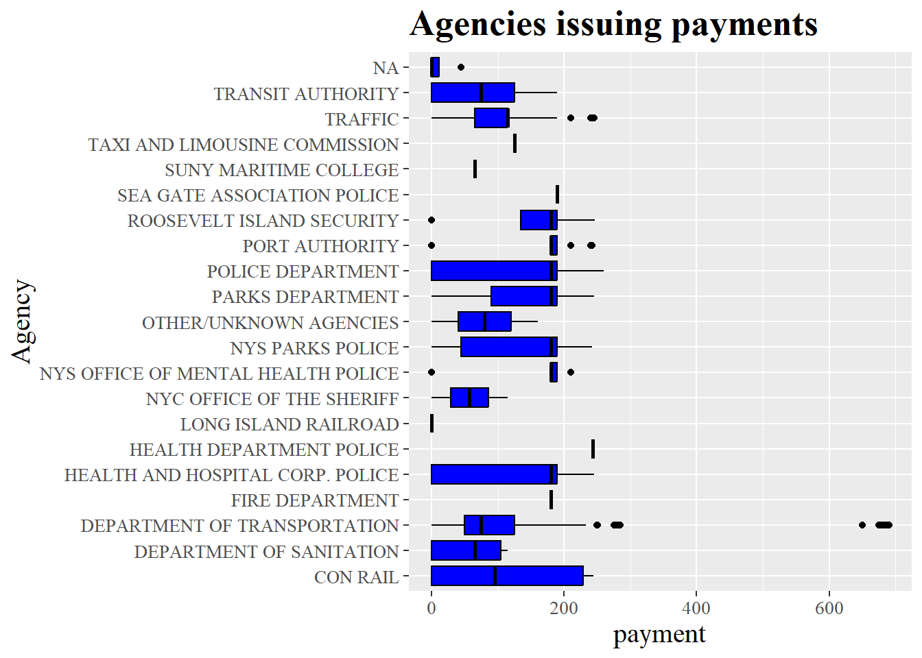
Figure 3.1: Boxplot showing issuing agency type by payment amount they give to people. Visualizing is helpful
3.4.5 Interpretation
The ANOVA performed showed that agency is statistically significant indicator for payment amount. Differences between the agencies are shown. The law firm might consider using the agency in their marketing strategy if they choose to look at agencies who have high payment amount.
3.5 Question 2: Do drivers from different states (NY, NJ, CT) pay more?
3.5.1 Descriptive Statistics
camera<- camera %>%
  filter(state %in% c("NY","NJ","CT"))

Drivers_Statistics<- favstats(payment_amount ~ state, data = camera) %>% arrange(desc(mean))

Drivers_Statistics
## state min Q1 median Q3 max mean sd n missing
## 1 NJ 0 50 75 115 682.35 101.5746 89.97170 8654 3
## 2 NY 0 50 75 125 690.04 101.0902 80.93015 79541 10
## 3 CT 0 50 75 100 276.57 80.6627 46.07849 1457 23.5.2 Inferential Statistics
##                Df    Sum Sq Mean Sq F value Pr(>F)
## state           2    602716  301358   45.48 <2e-16 ***
## Residuals   89649 594098897    6627
## ---
## Signif. codes:  0 '***' 0.001 '**' 0.01 '*' 0.05 '.' 0.1 ' ' 1
## 15 observations deleted due to missingness## Refitting to remove 15 cases with missing value(s)
## ℹ aov(formula = payment_amount ~ state, data = listwise_delete(camera,
## c("payment_amount", "state")))## Analysis of Variance Table (Type III SS)
## Model: payment_amount ~ state
##
## SS df MS F PRE p
## ----- --------------- | ------------- ----- ---------- ------ ----- -----
## Model (error reduced) | 602716.142 2 301358.071 45.475 .0010 .0000
## Error (from model) | 594098896.889 89649 6626.944
## ----- --------------- | ------------- ----- ---------- ------ ----- -----
## Total (empty model) | 594701613.031 89651 6633.5193.5.3 Interpretation
In the ANOVA we just conducted, the variance explained by the sum of squares using the formula SSerror/SStotal gives us 0.999. This sum of squares does account for a large amount of variance. The proportion of variance using the formula SSmodel/SStotal is 0.0007, which does not explain the variation portion of the data. The F value is 18.552 with a p value of .0000 which gives us a significant results. Drivers that come from different states do pay more.
3.5.4 Visualization
ggplot(camera, aes(x=state, y=payment_amount)) +
  geom_boxplot(fill = "orange", color = "black") +
  coord_flip() +
  labs(
    title ="Drivers payment by state",
    x="State",
    y="payment") +
  theme(plot.title = element_text(size=20, family="serif", face="bold"),
        axis.title = element_text(size=15, family ="serif"),
           axis.text = element_text(size = 10, family = "serif"))
## Warning: Removed 15 rows containing non-finite outside the scale range (`stat_boxplot()`).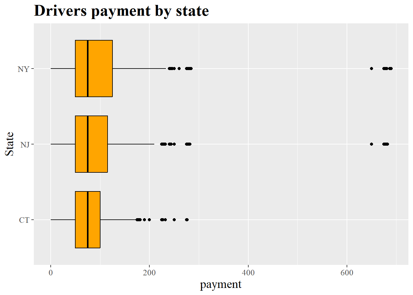
Figure 3.2: Boxplot showing drivers payment amoung by state
3.5.5 Interpretation
The ANOVA performed showed that Drivers from different states do pay higher, specifically those in New Jersey. State is statistically significant indicator for payment amount. Differences between the states payment amount are shown. The law firm should not really use this variable as it limits them to only certain states.
3.6 Question 3: Do certain counties tend to have higher payment amounts?
3.6.1 Descriptive Statistics
camera<- camera %>%
  filter(!is.na(county))

County_Statistics<- favstats(payment_amount ~ county, data = camera) %>% arrange(desc(mean))

County_Statistics
## county min Q1 median Q3 max mean sd n missing
## 1 Richmond County 0 65 180 180.0 245.79 138.80005 80.46141 811 0
## 2 Kings County 0 50 75 115.0 690.04 115.38500 132.61340 14184 0
## 3 Monroe County 0 50 75 150.0 280.38 102.46441 74.50960 13476 0
## 4 Bronx County 0 65 85 167.5 245.64 101.71333 66.51450 222 0
## 5 New York County 0 65 115 115.0 260.00 91.60696 38.32289 8144 0
## 6 Queens County 0 50 50 100.0 283.03 84.12366 60.74257 15897 0
## 7 Staten Island County 0 50 50 75.0 250.00 67.43513 41.86493 425 03.6.2 Inferential Statistics
##                Df    Sum Sq Mean Sq F value Pr(>F)
## county          6   9642588 1607098   212.6 <2e-16 ***
## Residuals   53152 401810433    7560
## ---
## Signif. codes: 0 '***' 0.001 '**' 0.01 '*' 0.05 '.' 0.1 ' ' 1## Analysis of Variance Table (Type III SS)
## Model: payment_amount ~ county
##
## SS df MS F PRE p
## ----- --------------- | ------------- ----- ----------- ------- ----- -----
## Model (error reduced) | 9642588.258 6 1607098.043 212.589 .0234 .0000
## Error (from model) | 401810432.597 53152 7559.648
## ----- --------------- | ------------- ----- ----------- ------- ----- -----
## Total (empty model) | 411453020.854 53158 7740.1903.6.3 Interpretation
In the ANOVA we just conducted, the variance explained by the sum of squares using the formula SSerror/SStotal gives us 0.977. This sum of squares does account for a large amount of variance. The proportion of variance using the formula SSmodel/SStotal is 0.02, which does not explain for a large variation portion of the data. The F value is 212.589 with a p value of .0000 which gives us a significant results. Some counties do tend to have higher payment amounts.
3.6.4 Visualization
ggplot(camera, aes(x=county, y=payment_amount)) +
  geom_boxplot(fill = "green", color = "black") +
  coord_flip() +
  labs(
    title ="County Payment Amounts",
    x="County",
    y="payment") +
  theme(plot.title = element_text(size=20, family="serif", face="bold"),
        axis.title = element_text(size=15, family ="serif"),
           axis.text = element_text(size = 10, family = "serif"))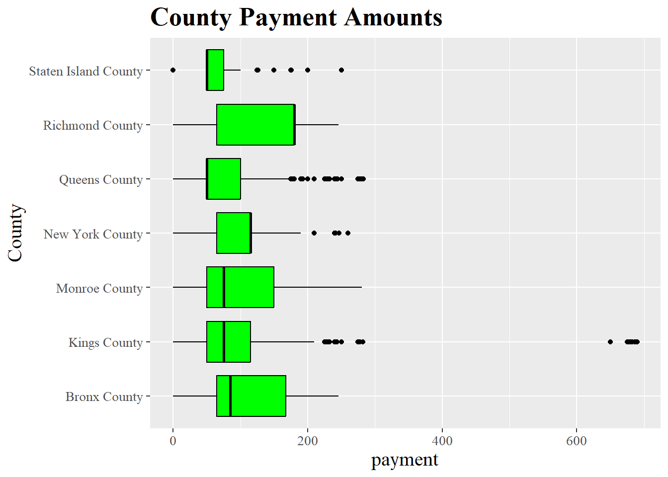
Figure 3.3: Boxplot showing payment amount by county
3.6.5 Interpretation
The ANOVA performed showed that different counties tend to have higher payment amounts, specifically Richmond County. The county variable is a statistically significant indicator for payment amount. Differences between the county payment amount are shown. The law firm should use this variable to investigate further which counties have the highest payment and use in their marketing strategies.